Traders Lost in the Hedge Maze

I recently wrote five short essays on the subtle art of derivative hedging.

Financial mathematics is often done under highly idealised assumptions, especially at the introductory level. This is unfortunate since students can leave academic programs with a somewhat disconnected understanding of the practical nature of financial engineering. In the referenced notebook I endeavour to walk a fine line between academia and industry, exploring one of the most fundamental aspects of derivatives trading - hedging - in five easy pieces. Specifically, I strive for a kind of quasi- (or pseudo-) realism, where simulated data is considered, but a subset of the original Black-Scholes-Merton assumptions gradually are alleviated.

In Delta Hedging at Discrete Intervals I explore the effects of hedging a finite number of times: what error do we accrue vis-a-vis hedging in a continuous time economy?
In Gamma Hedging at Discrete Intervals I extend the previous essay by hedging the second order sensitivity to the underlying with another derivative. What impact does this have on the hedge error?
In Hedging with Volatility Uncertainty I dismiss the idea that implied, realised, and hedging volatilities are all equal. What happens to the PnL of our hedge portfolio when these are allowed to be different?
In Hedging with Transaction Costs I banish the frictionless economy while seeking a notion of ‘optimal hedging’.
Finally, in Risk Minimising Hedges I consider how necessarily imperfect hedges nonetheless can be made as good as possible, focusing on the case of stochastic volatility.

These are all known theoretical results, but regrettably they remain obscure to many who ought to know.
My contribution here is purely expository. Also: you are unlikely to find this stuff coded up anywhere else, so here you go:

“To read the five essays please click here. The link takes you to a Jupyter Notebook hosted on Github.”

For a sample of the Notebook, I provide an abridged (code free) version of the first chapter below:

Ch. 1: Delta Hedging at Discrete Intervals

Black and Scholes famously demonstrated that the price process of a call option \(C_t = C_t(K,T)\) is perfectly replicable by dynamically adjusting a self-financing position in nothing but a risk-free bank account \(B_t\) and the underlying security \(S_t\). However, the conditions under which this is true are notoriously incredulous: for example, market are manifestly not free from transaction costs and nobody can adjust a portfolio continuously in time.

So traders adjust their portfolios at discrete intervals \(\mathbb{T} = \{t_1, t_2, ..., t_n\}\), thereby inducing some measure of hedge error. How stark is the discrepancy? To answer this question, let us first consider where a discretely rebalanced hedge portfolio ends up vis-a-vis the terminal payoff under \(M\) different simulated stock paths. We consider initialising a hedge portfolio \(\Pi = B + \Delta S\) such that at time 0, the value is equivalent to the call option \(C_0\). For each \(t \in \mathbb{T}\) we re-balance the portfolio, adjusting the position in the stock to be that of the relevant Black-Scholes delta at the time. This rebalancing is done in a self-financing manner, meaning that the value of the portfolio just after the rebalancing, is identical to the value of the portfolio just before the rebalancing. Formally, the position in the bank at rebalancing time \(t_{i}^+\) must satisfy the equation

\[B_{t_{i}^-} + \Delta_{t_{i}^-} S_{t_{i}^-} = B_{t_{i}^+} + \Delta_{t_{i}^+} S_{t_{i}^+} \Longleftrightarrow B_{t_{i-1}}e^{r (t_i-t_{i-1})} + \Delta_{t_{i-1}} S_{t_{i}} = B_{t_i} + \Delta_{t_i} S_{t_{i}}.\]

Suppose we simulate \(M=500\) geometric Brownian motion paths with the following parameter specifications:

S_0 = 100  # spot
K = 110  # strike
τ = 1  # time to maturity
μ = 0.1  # mean drift
σ = 0.2  # volatility
r = 0.01  # risk free rate

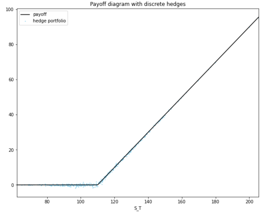
If we use these paths to form \(M\) self-financing portfolios rebalanced once per day, we can compare the terminal value of the hedge portfolio \(\Pi_T\) with the option pay-off \(C_T = \max\{S_T-K,0 \}\). Doing so, I get the plot below.

Rejoice! The discrete hedge matches the option payoff to a good degree of accuracy, with the bulk of discrepancies lying around the at-the-money point (unsurprising: recall \(\Delta\) converges to \(\mathbb{1}\{S_T \geq K\}\) at maturity, meaning that it is easy to get the delta wrong around this point).

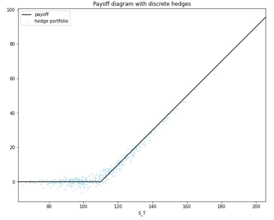
How badly does this deteriorate if we decrease the hedge frequency - e.g. by switching to a ‘once every 21 days’ rebalancing scheme? The figure below gives some intuition: the hedge portfolios are markedly more off-target, but not comically so.

To uncover the relationship between hedge frequencies and hedge errors, it is instructive to run this experiment for a range of hedge intervals, computing the standard deviation of the hedge error \((\Pi_T - C_T)\) in each case. In the plot below I consider hedging once every \(\{1, 3, 5, 7, 14, 21, 42, 63 \}\) days:

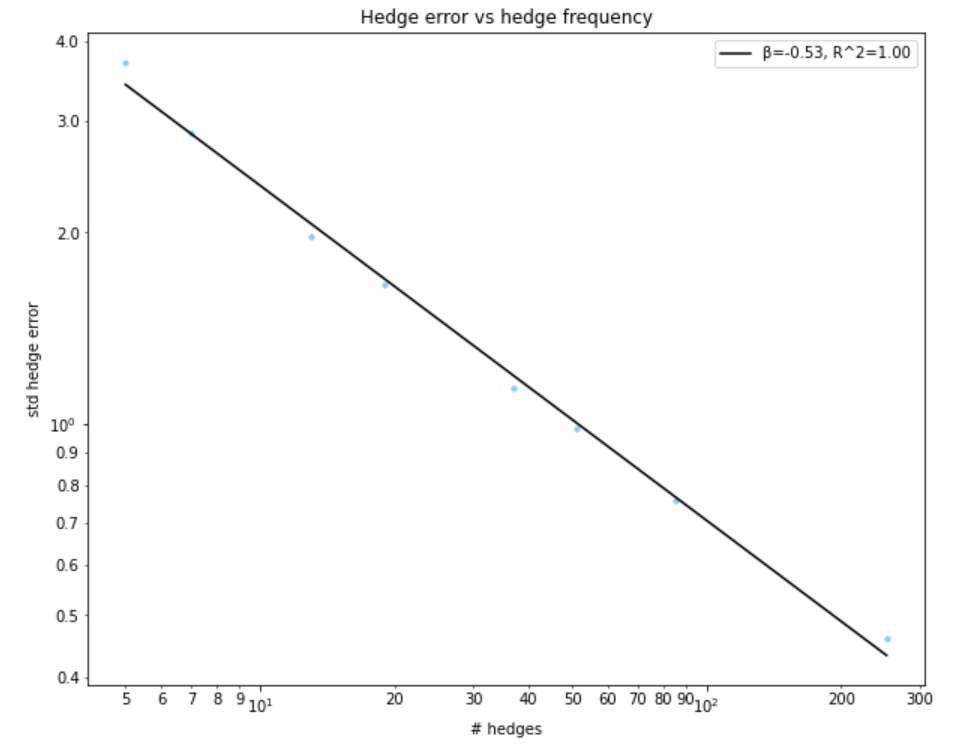
Based on this log-log plot we conclude that the hedge error scales as one over the square root of the number of hedges performed during the lifetime of the option (\(R^2 \approx 1\)). I.e. when you quadruple your hedge frequency you halve your hedge error.

Can we show this formally? Yes! It’s slightly hairy, but the argument runs along the following lines: consider the hedge error \(\epsilon_{\delta t}\) that arises between an option and a replicating portfolio \(\Pi = B+\Delta S\) over some discrete interval \(\delta t\):

\[\begin{aligned} \epsilon_{\delta t} & \equiv \delta C - \delta\Pi \\ &=\delta C - \delta (B + \Delta S) \\ &\approx \delta C - r B \delta t - \Delta \delta S \\ &= \delta C - r (C-\Delta S) \delta t - \Delta \delta S. \end{aligned}\]

Now \(\delta S = \mu S \delta t + \sigma S \sqrt{\delta t} Z\), where \(Z \sim N(0,1)\), and by Itô \(\delta C \approx \theta \delta t + \Delta \delta S + \tfrac{1}{2} \Gamma (\delta S)^2\). Substituting these expression into the above, and ignoring terms \(O(\delta t^2)\) we obtain

\[\begin{aligned} \epsilon_{\delta t} &\approx (\theta - rC + r \Delta S ) \delta t + \tfrac{1}{2} \Gamma \sigma^2 S^2 Z^2 \delta t \\ &= \tfrac{1}{2} \Gamma \sigma^2 S^2 (Z^2 - 1) \delta t, \end{aligned}\]

where the second line has made use of the Black-Scholes PDE: \(rC = \theta + r\Delta S + \tfrac{1}{2} \sigma^2 S^2 \Gamma\). The cumulative hedge error from discrete hedging over the lifetime of the option is therefore

\[\epsilon \approx \sum_{i=1}^n \tfrac{1}{2} \Gamma_i \sigma^2 S_i^2 (Z_i^2 - 1) \delta t,\]

where \(\Gamma_i\) is understood to be the gamma at time \(t_i\) (ttm \(T-t_i\)) when spot is \(S_i\). By iterated expectations this has expectation 0 (recall \(\mathbb{E}[Z^2]=1\)). Meanwhile the variance of the hedge error is approximately

\[\mathbb{V}[\epsilon] \approx \mathbb{E} \left[ \sum_{i=1}^n \tfrac{1}{2} (\Gamma_i S_i^2)^2 (\sigma^2 \delta t)^2 \right]\]

since \(\mathbb{E}[(Z^2-1)^2] = \mathbb{E}[Z^4-2Z^2+1] = 3-2+1 = 2\). Evaluating this requires some effort. Derman and Miller provide (some) of the hard work (see eqns. (6.8) and (6.9)) if you are interested. Here, the upshot will do:

\[\mathbb{V}[\epsilon] \approx \sum_{i=1}^n \tfrac{1}{2} S_0^4 \Gamma_0^2 \sqrt{\frac{T^2}{T^2-t_i^2}} (\sigma^2 \delta t)^2 \approx \frac{\pi}{4} n (S_0^2 \Gamma_0 \sigma^2 \delta t)^2,\]

where \(n \equiv (T-t)/\delta t\). Finally, it is well known that gamma can be expressed as vega through \(S_0^2 \Gamma_0 \sigma (T-t) = \nu\). Using this fact, we arrive at

\[\mathbb{V}[\epsilon] \approx \frac{\pi}{4n} (\sigma \nu)^2 \Longrightarrow \text{std}(\epsilon) \approx \frac{\sigma}{\sqrt{n}} \nu\]

which is the \(\propto 1/\sqrt{n}\) relationship we wanted to show.

Want More?

To read all five essays with Python code, click here.