Sub-optimal Optimal Portfolios
A perfect Brownian
Imagine you are truthfully told about the functional form of the stochastic equations of motion characterising some set of stocks, with the caveat that you are required to estimate the associated parameters yourself. Prima facie, this complete removal of Knightian uncertainty sounds like a dream scenario which trivially will allow for what we vaguely can call “perfect trading”. In this piece I want to convince you that things are not quite so straight-forward. In particular, even with a substantial amount of data at your disposal, parameter uncertainty can still undermine theoretically optimal strategies. To cement this point, I will consider the simulated performance of a number of results from modern portfolio theory, both in the event that we do and do not have complete information about the input parameters. In a certain sense, this analysis is befitting considering that the father of modern portfolio theory, Harry Markowitz, famously doesn’t practice what he preaches, being instead partial towards “equal weight” diversification.
To set the scene, let us suppose that the daily percentage returns of \(K\) assets are multivariate normal, \(\boldsymbol{R}_t \sim \mathcal{N}(\boldsymbol{\mu} \Delta t, \boldsymbol{\Sigma} \Delta t)\), where \(\boldsymbol{\mu} \in \mathbb{R}^K\) is an annualised mean return vector, and \(\boldsymbol{\Sigma} \in \mathbb{R}^{K \times K}\) is an annualised covariance matrix i.e. \(\boldsymbol{\Sigma} \equiv \text{diag}(\boldsymbol{\sigma})\boldsymbol{\varrho}\text{diag}(\boldsymbol{\sigma})\) where \(\boldsymbol{\sigma} \in \mathbb{R}^K\) is a volatility vector, and \(\boldsymbol{\varrho} \in \mathbb{R}^{K \times K}\) is a correlation matrix. \(\Delta t\) scales these quantities into daily terms and is typically set to 1/252 to reflect the average number of trading days in a year.
Equivalently, we may write this in price process terms as the dynamics
\[\boldsymbol{S}_{t+1} = \boldsymbol{S}_{t} + \text{diag}(\boldsymbol{S}_{t})(\boldsymbol{\mu} \Delta t + \boldsymbol{L} \sqrt{\Delta t} \boldsymbol{Z}),\]where \(\boldsymbol{L}\) is the lower triangular matrix arising from Cholesky decomposing \(\boldsymbol{\Sigma}\), and \(\boldsymbol{Z}: \Omega \mapsto \mathbb{R}^K\) is an i.i.d. standard normal vector i.e \(\boldsymbol{Z} \sim \mathcal{N}(\boldsymbol{0}, \mathbb{I}_{K})\).
For the purpose of this exercise we shall consider five co-moving assets with the following parameter specifications:
μ = np.array([0.1, 0.13, 0.08, 0.09, 0.14]) #mean
σ = np.array([0.1, 0.15, 0.1, 0.1, 0.2]) #volatility
ρ = np.array([[1, 0, 0, 0, 0],
              [0.2, 1, 0, 0, 0],
              [0.3, 0.5, 1, 0, 0],
              [0.1, 0.2, 0.1, 1, 0],
              [0.4, 0.1, 0.15, 0.2, 1]])
ρ = ρ+ρ.T-np.identity(len(μ)) #correlation
dt = 1/252 #1/trading days per year
T = 10 #simulation time [years]
r = 0 #risk-free rate
S_0 = 100*np.ones(len(μ)) #initial share prices
W_0 = 1e6 #initial welath
Furthermore, it will be convenient to define the following quantities:
M = len(μ)
N = int(T/dt)
Σ = np.diag(σ)@ρ@np.diag(σ)
Σinv = np.linalg.inv(Σ)
sqdt = np.sqrt(dt)
λ, Λ = np.linalg.eig(Σ)
assert (λ > 0).all() #assert positive semi-definite
L = np.linalg.cholesky(Σ)
I = np.ones(M)
Sharpe = (μ-r)/σ
Finally, to simulate stock paths according to these inputs we can use the following vectorised function:
def multi_brownian_sim(seed: bool = False) -> Tuple[pd.DataFrame, pd.DataFrame]:

    if seed:
        np.random.seed(42)
    dW = pd.DataFrame(np.random.normal(0, sqdt, size=(M, N+1)))
    ret = (1 + L@dW + np.tile(μ*dt, (N+1,1)).T)
    ret = ret.T
    ret.iloc[0] = S_0
    df = ret.cumprod() #levels
    dfr = (df.diff()/df.shift(1)).dropna() #returns

    return df, dfr
A single run of this yields something along the lines below:
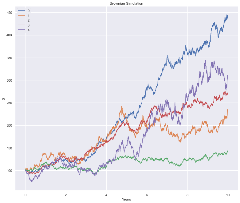
Estimating parameters
Alright, suppose you are handed the data for these paths above and informed that returns are multivariate normal. What do you conclude? Well, you’ll probably find the unbiased estimators \(\{\hat{\boldsymbol{\mu}}, \hat{\boldsymbol{\sigma}}, \hat{\boldsymbol{\varrho}} \}\) as displayed in the 2nd column in the tables below. The noteworthy part here is how much some of these appear amiss vis-à-vis their population counterparts. So much so that one almost suspects that something is messed up with the data-generating process per se. To assure you this is not the case, we will do a couple of exercises: first, we will compute two-sigma confidence intervals for our estimators, and second, we will sample from the data-generating process repeatedly and show that the averages over the estimators indeed are congruent with the true underlying dynamics.
Confidence intervals for \(\hat{\boldsymbol{\mu}}\) and \(\hat{\boldsymbol{\sigma}}^2\) can be computed using the central limit theorem: indeed, it is straightforward to show that \(\sqrt{N}(\hat{\mu}_i - \mu_i) \sim \mathcal{N}(0, \sigma_i^2)\) and \(\sqrt{N}(\hat{\sigma}_i^2 - \sigma_i^2) \sim \mathcal{N}(0, 2\sigma_i^4)\) where \(N\) is the number of observations. Deploying the delta method to extract the limiting distribution of \(\hat{\boldsymbol{\sigma}}\) we find that \(\sqrt{N}(\hat{\sigma}_i - \sigma_i) \sim \mathcal{N}(0, \sigma_i^2/2)\). Finally, confidence intervals for \(\hat{\varrho}_{ij}\) can be estimated using the Fisher transformation.
For the Monte Carlo simulation we run the data generating process 1000 times storing the estimators for \(\{\hat{\boldsymbol{\mu}}, \hat{\boldsymbol{\sigma}}, \hat{\boldsymbol{\varrho}} \}\) from each run in order to ultimately study their statistical properties. Per definition, 95% of the confidence intervals we’d compute from repeated sampling should encompass the true population parameters. Notice the expected values (6th column) across these samples align much more closely with the true parameters: a small victory for having the equivalent of 10,000 years’ worth of financial data(!)
| $$\mu$$ | $$\hat{\mu}$$ | $$\hat{\mu}-2SE$$ | $$\hat{\mu}+2SE$$ | $$\in CI$$ | $$\mathbb{E}(\mu_{mc})$$ | $$\min(\mu_{mc})$$ | $$\max(\mu_{mc})$$ | |
|---|---|---|---|---|---|---|---|---|
| 0 | 0.10 | 0.152 | 0.090 | 0.214 | True | 0.097 | 0.003 | 0.191 |
| 1 | 0.13 | 0.096 | -0.000 | 0.192 | True | 0.131 | -0.035 | 0.252 |
| 2 | 0.08 | 0.039 | -0.024 | 0.103 | True | 0.080 | -0.027 | 0.173 |
| 3 | 0.09 | 0.105 | 0.043 | 0.168 | True | 0.089 | -0.019 | 0.197 |
| 4 | 0.14 | 0.132 | 0.007 | 0.257 | True | 0.139 | -0.039 | 0.339 |
| $$\sigma$$ | $$\hat{\sigma}$$ | $$\hat{\sigma}-2SE$$ | $$\hat{\sigma}+2SE$$ | $$\in CI$$ | $$\mathbb{E}(\sigma_{mc})$$ | $$\min(\sigma_{mc})$$ | $$\max(\sigma_{mc})$$ | |
|---|---|---|---|---|---|---|---|---|
| 0 | 0.10 | 0.098 | 0.096 | 0.101 | True | 0.10 | 0.096 | 0.104 |
| 1 | 0.15 | 0.152 | 0.147 | 0.156 | True | 0.15 | 0.144 | 0.158 |
| 2 | 0.10 | 0.101 | 0.098 | 0.104 | True | 0.10 | 0.096 | 0.104 |
| 3 | 0.10 | 0.099 | 0.096 | 0.101 | True | 0.10 | 0.095 | 0.104 |
| 4 | 0.20 | 0.198 | 0.192 | 0.203 | True | 0.20 | 0.191 | 0.208 |
| $$\rho$$ | $$\hat{\rho}$$ | $$\hat{\rho}-2SE$$ | $$\hat{\rho}+2SE$$ | $$\in CI$$ | $$\mathbb{E}(\rho_{mc})$$ | $$\min(\rho_{mc})$$ | $$\max(\rho_{mc})$$ | ||
|---|---|---|---|---|---|---|---|---|---|
| 0 | 1 | 0.20 | 0.208 | 0.169 | 0.245 | True | 0.200 | 0.146 | 0.260 |
| 2 | 0.30 | 0.292 | 0.256 | 0.328 | True | 0.299 | 0.233 | 0.365 | |
| 3 | 0.10 | 0.057 | 0.017 | 0.096 | False | 0.100 | 0.039 | 0.159 | |
| 4 | 0.40 | 0.405 | 0.371 | 0.438 | True | 0.400 | 0.340 | 0.456 | |
| 1 | 2 | 0.50 | 0.483 | 0.452 | 0.513 | True | 0.500 | 0.447 | 0.545 |
| 3 | 0.20 | 0.189 | 0.151 | 0.227 | True | 0.200 | 0.137 | 0.256 | |
| 4 | 0.10 | 0.138 | 0.099 | 0.177 | True | 0.100 | 0.037 | 0.163 | |
| 2 | 3 | 0.10 | 0.124 | 0.085 | 0.163 | True | 0.101 | 0.043 | 0.164 |
| 4 | 0.15 | 0.179 | 0.140 | 0.217 | True | 0.150 | 0.093 | 0.208 | |
| 3 | 4 | 0.20 | 0.199 | 0.160 | 0.237 | True | 0.200 | 0.139 | 0.261 |
Scanning through the above numbers the most problematic estimator is clearly \(\hat{\boldsymbol{\mu}}\). Intuitively, we can explain this as follows: since \(R_t \equiv (S_t-S_{t-1})/S_{t-1} \approx \ln(S_t)-\ln(S_{t-1})\) it follows that
i.e. the estimator is a telescoping series effectively determined by the first and last entry. For “shorter” histories this can be extremely problematic (noisy).
The final frontier?
To get a sense of the sheer amount of gravity these uncertainties carry, it is helpful to consider the efficient frontier i.e. the collection of portfolio constructions which deliver the lowest amount of volatility for a given level of return. A well known result in modern portfolio theory states that this frontier carves out a hyperbola in (standard deviation, mean)-space given by the equation
\[\sigma_{\pi}^2(\mu_{\pi}) = \frac{C \mu_{\pi}^2 - 2B \mu_{\pi} + A}{D},\]where \(A \equiv \boldsymbol{\mu}^\intercal \boldsymbol{\Sigma}^{-1} \boldsymbol{\mu}\), \(B \equiv \boldsymbol{\mu}^\intercal \boldsymbol{\Sigma}^{-1} \boldsymbol{1}\), \(C \equiv \boldsymbol{1}^\intercal \boldsymbol{\Sigma}^{-1} \boldsymbol{1}\), and \(D \equiv AC-B^2\).
The function below allows us to visualise the efficient frontier for arbitrary \(\boldsymbol{\mu}\), \(\boldsymbol{\Sigma}\):
def plot_frontier(μ_est: np.array, Σ_est: np.array, ax = None, scatter: bool = False, muc: float = 0.3, alpha: float = 0.5):

    σ_est = np.sqrt(np.diag(Σ_est))
    Σinv_est = np.linalg.inv(Σ_est)

    A = μ_est@Σinv_est@μ_est
    B = μ_est@Σinv_est@I
    C = I@Σinv_est@I
    D = A*C - B**2
    if μ_est.max() > muc:
        muc = μ_est.max() + 0.1
    mubar = np.arange(0,muc,0.005)
    sigbar = np.sqrt((C*pow(mubar,2) - 2*B*mubar + A)/D)

    if ax == None:
        fig, ax = plt.subplots(1,1, figsize=(13,11))

    ax.plot(sigbar, mubar, alpha=alpha)
    if scatter:
        ax.scatter(σ_est, μ_est)
    ax.set_xlabel(r'$\sigma$')
    ax.set_ylabel(r'$\mu$')
    ax.set_title('Efficient Frontier')
E.g. for the specified parameters characterising the five assets, this yields the following curve:
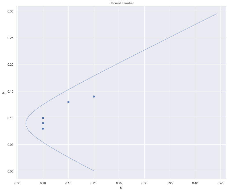
Now let’s consider what happens if \(\boldsymbol{\mu}\) is known a priori, but \(\boldsymbol{\Sigma}\) must be estimated from the data. As above, we’ll repeat the data generating process 1000 times, recomputing the frontier on each iteration, to get a sense of the variability.
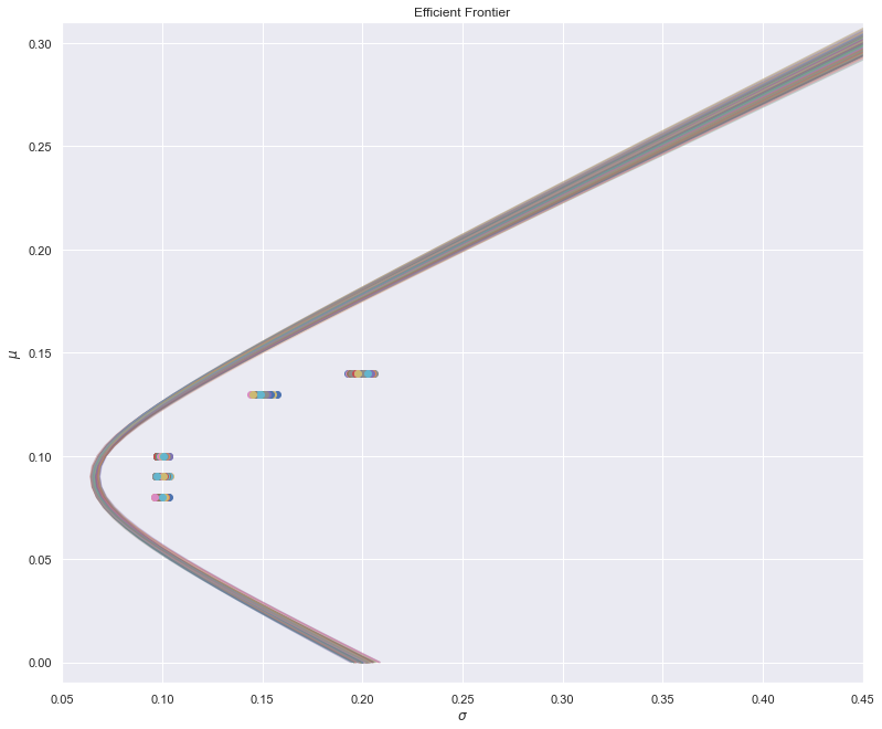
Evidently, while this introduces some estimation error, the overall picture remains “within reason”.
Finally, suppose both \(\boldsymbol{\mu}\) are \(\boldsymbol{\Sigma}\) are inferred a posteriori. The Monte Carlo run yields:
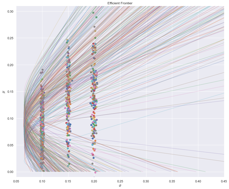
… which isn’t exactly great.
The question remains: to what extent does this actually impact quantitative trading strategies? Well, the efficient frontier does include a couple of portfolios of interest, most notably the minimum variance portfolio and the maximum Sharpe ratio portfolio, both of which plausibly could be adopted by practitioners. Let’s see how such strategies fare in light of our current framework.
One-period “optimal” trading strategies
One of the great tragedies of academic finance is the curious disconnect with which it operates from the practical field. Optimisation, for example, is a major division of mathematical finance, yet empirical tests thereof are shockingly scarce. So much so that the enfant terrible of the quant industry, Nassim Taleb, noted in “The Black Swan”:
“I would not be the first to say that this optimisation set back the social science by reducing it from the intellectual and reflective discipline it was becoming to an attempt at an “exact science”. By “exact science”, I mean a second-rate engineering problem for those who want to pretend that they are in a physics department - so-called physics envy. In other words, an intellectual fraud”.
To remedy this deplorable situation, let us finally explore how optimal one-period portfolio constructions fare against equal allocation (\(1/K\) diversification). In particular, let us consider whether (I) the minimum variance portfolio1:
\[\boldsymbol{\pi}_{\text{minvar}} = \frac{\boldsymbol{\Sigma}^{-1} \boldsymbol{1}}{ \boldsymbol{1}^\intercal \boldsymbol{\Sigma}^{-1} \boldsymbol{1}},\]actually delivers a smaller variance than the \(1/K\) benchmark. For reference: \(\boldsymbol{\pi}_{\text{minvar}} \approx (0.32, 0.00, 0.31 , 0.38, -0.01)\). Similarly whether (II) the maximum sharpe ratio portfolio2:
\[\boldsymbol{\pi}_{\text{maxshp}} = \frac{\boldsymbol{\Sigma}^{-1} (\boldsymbol{\mu}-r\boldsymbol{1})}{ \boldsymbol{1}^\intercal \boldsymbol{\Sigma}^{-1} (\boldsymbol{\mu}-r\boldsymbol{1})},\]actually delivers a higher Sharpe ratio than the \(1/K\) benchmark. For reference: \(\boldsymbol{\pi}_{\text{maxshp}} \approx (0.34, 0.14, 0.14, 0.33, 0.05)\).
To analyse these questions, consider the following experimental set-up: Using simulated data we will run five self-financing portfolios for 10 years, each starting with a million dollar notational. The five strategies under scrutiny are: (i) The \(1/K\) portfolio, (ii) \(\boldsymbol{\pi}_{\text{minvar}}\) with known parameters, (iii) \(\boldsymbol{\pi}_{\text{minvar}}\) with unknown parameters, (iv) \(\boldsymbol{\pi}_{\text{maxshp}}\) with known parameters, and (v) \(\boldsymbol{\pi}_{\text{maxshp}}\) with unknown parameters. All estimated quantities will be based on at least ten years’ worth of history and will be updated weekly. At the end all portfolios will have their variance and Sharpe ratio computed. As usual, we’ll repeat this entire process 1000 times.
For a given matrix of simulated returns, the following function computes the wealth paths of the five strategies:
π_eql = np.ones(M)/M #equally weighted portfolio
π_var = (Σinv@I)/(I@Σinv@I) #minimum variance portfolio
π_shp = (Σinv@(μ-r))/(I@Σinv@(μ-r)) #optimal sharpe portfolio

def wealth_path(dfr: pd.DataFrame) -> Tuple[pd.DataFrame, pd.DataFrame, pd.DataFrame]:

    col = ['W_equal', 'W_minvar', 'W_minvar_est', 'W_sharpe', 'W_sharpe_est',]
    t_test = np.arange(int(N/2),N+1)
    dfw = pd.DataFrame(np.nan, index=t_test,columns=col)
    dfw.loc[t_test[0],:] = W_0
    pi_shp_dic = {}
    pi_var_dic = {}

    μ_hat_vec = dfr.expanding().mean()/dt
    Σ_hat_vec = dfr.expanding().cov()/dt

    for ti, t in enumerate(t_test):
        if ti%7 == 0:
            μ_hat = μ_hat_vec.loc[t].values
            Σ_hat = Σ_hat_vec.loc[t].values
            Σinv_hat = np.linalg.inv(Σ_hat)
            pi_shp_dic[t] = (Σinv_hat@(μ_hat-r))/(I@Σinv_hat@(μ_hat-r))
            pi_var_dic[t] = (Σinv_hat@I)/(I@Σinv_hat@I)
        else:
            pi_shp_dic[t] = pi_shp_dic[t-1]
            pi_var_dic[t] = pi_var_dic[t-1]

        if ti == 0:
            pass
        else:
            col_map = {
                'W_equal': π_eql,
                'W_minvar': π_var,
                'W_minvar_est': pi_var_dic[t-1],
                'W_sharpe': π_shp,
                'W_sharpe_est': pi_shp_dic[t-1],
            }
            for j in col:
                dfw.at[t,j] = dfw.at[t-1,j]*(1 + col_map[j]@dfr.loc[t])

    pi_shp = pd.DataFrame.from_dict(pi_shp_dic, orient='index')
    pi_var = pd.DataFrame.from_dict(pi_var_dic, orient='index')
    return dfw, pi_shp, pi_var
Here’s one such example, which in itself won’t tell you much:
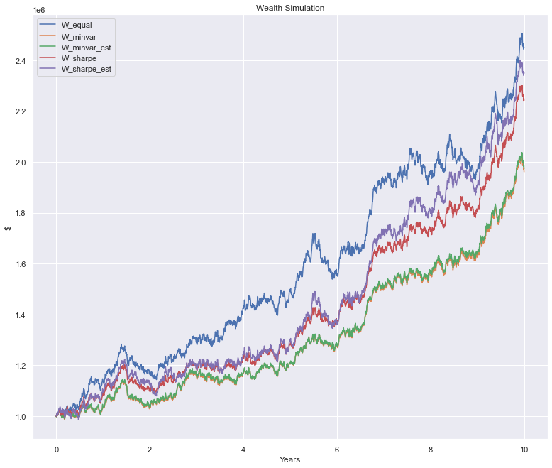
However, once we repeat this enough times a pattern starts to emerge. Specifically, consider the distributive properties of the optimal portfolios less the \(1/K\) benchmark:
| $$\sigma(\boldsymbol{\pi}_{\text{minvar}})-\sigma(\boldsymbol{\pi}_{1/K} )$$ | $$\sigma(\hat{\boldsymbol{\pi}}_{\text{minvar}})-\sigma(\boldsymbol{\pi}_{1/K} )$$ | $$Shp(\boldsymbol{\pi}_{\text{maxshp}})-Shp(\boldsymbol{\pi}_{1/K} )$$ | $$Shp(\hat{\boldsymbol{\pi}}_{\text{maxshp}})-Shp(\boldsymbol{\pi}_{1/K} )$$ | |
|---|---|---|---|---|
| count | 1000 | 1000 | 1000 | 1000 |
| mean | -0.015 | -0.015 | 0.104 | 0.008 |
| std | 0.001 | 0.001 | 0.120 | 0.161 |
| min | -0.018 | -0.018 | -0.299 | -0.790 |
| 2.5% | -0.017 | -0.017 | -0.119 | -0.308 |
| 50% | -0.015 | -0.015 | 0.105 | 0.003 |
| 97.5% | -0.013 | -0.013 | 0.342 | 0.352 |
| max | -0.013 | -0.013 | 0.503 | 0.641 |
| # < 0 | 1000 | 1000 | 200 | 493 |
The take-away here is that the minimum variance portfolio does, in fact, deliver a lower volatility than the equal allocation portfolio - regardless of whether \(\boldsymbol{\Sigma}\) is estimated or not. As for the maximum Sharpe ratio portfolio the situation is more problematic: while 80% of the portfolios with known parameters do outperform the benchmark, there’s little to suggest optimisation actually helps once we introduce estimation into the picture. Again, the culprit is the uncertainty around the \(\hat{\boldsymbol{\mu}}\) estimator.
In summary, even under highly idealised circumstances optimal trading strategies may not deliver as expected. Indeed, I would strongly caution against embracing small improvements in portfolio performance from some complicated optimisation process vs. keeping things simple. Markowitz’s \(1/K\) portfolio allocation is a lot less irrational than it initially appears.
-
I.e. the solution to \(\min_{\boldsymbol{\pi}} \boldsymbol{\pi}^\intercal \boldsymbol{\Sigma} \boldsymbol{\pi}\) where \(\boldsymbol{\pi}^\intercal \boldsymbol{1}=1\). ↩
-
I.e. the solution to \(\max_{\boldsymbol{\pi}} (\boldsymbol{\pi}^\intercal\mu - r)/\sqrt{\boldsymbol{\pi}^\intercal \boldsymbol{\Sigma} \boldsymbol{\pi}}\) where \(\boldsymbol{\pi}^\intercal \boldsymbol{1}=1\). ↩