The SVI Model - A Tutorial
When a smile means the world: in the Bhagavata Purana, Krishna famously gives his foster mother a glimpse of his true essence (“Vishvarupa”) in a most unusual manner. At a more pedestrian level the ‘world’ is also baked into the volatility smile which codifies the market view of the (risk neutral) distributive properties of the underlying security.
The SVI model: The theoretical minimum.
The Stochastic Volatility Inspired (SVI) model is a parametric equation for the volatility smile designed by Jim Gatheral during his time at Merrill Lynch in the late 1990s. Several highly readable theoretical expositions exist including Gatheral , Gatheral and Jacquier, and Ferhati, which you are encouraged to consult. In this piece we provide a self-contained introduction to the subject, focussing on implementation: the theory is deliberately kept cursory. Note that I’ve only run this code ad hoc, and make no claims of it being production grade. If you find anything untoward, let me know.
The core idea of the SVI can be summarised as follows: rather than fitting a global model of the volatility surface in “one go” the SVI model sets out to fit each smile individually (one expiry date at a time), often with careful constraints applied to ensure that all smiles preclude arbitrage. Specifically, for a given tenor \(\tau\), the SVI model postulates that the smile be modelled as
\[w(k,\tau) = a + b \left\{ \varrho (k-m) + \sqrt{(k-m)^2 + \sigma^2} \right\},\]where \(w: \mathbb{R} \times [0,T] \mapsto \mathbb{R}^+\) is the total variance, defined as \(w(k,\tau) \equiv \tau \sigma_{BS}^2(k,\tau)\) (the time scaled Black Scholes implied vol squared) and \(k\) is the log forward moneyness, defined as \(\ln(K/F_\tau)\), where \(K\) and \(F_\tau\) are the strike and forward prices. For ease of notation we have suppressed the \(\tau\) dependence on the parameters \(\chi \equiv \{a,b,\varrho, m, \sigma\}\), but keep this in mind. Roughly speaking, \(a \in \mathbb{R}\) controls the overall variance level (vertical translations); \(b \in \mathbb{R}^+\) controls the slope of the wings; \(\varrho \in (-1,1)\) controls the counter-clockwise rotation of the smile; \(m \in \mathbb{R}\) the vertical translations, and \(\sigma \in \mathbb{R}^+\) the level of curvature.
Further constraints must be enforced upon the parameters to ensure sensible results. For starters Gatheral lists the requirement that \(a+b \sigma \sqrt{1-\varrho^2} \geq 0\) for a non-negative total variance. More subtle constraints arise from eliminating arbitrage. E.g. on the intra-smile level, the absence of butterfly arbitrage entails that one cannot go long a fly (option structure) without paying for the pleasure. (A fly has a pay-off structure which is everywhere non-negative. You don’t get this sort of optionality for free). By Breeden Litzenberger this turns out to be equivalent to requiring that the risk neutral density function is everywhere non-negative (a very reasonable disposition indeed). A tedious argument shows that this amounts to requiring that \(g(k) \geq 0\), \(\forall k\) where we have defined
\[g(k) \equiv \left( 1-\frac{kw'(k)}{2w(k)} \right)^2 - \frac{w'(k)^2}{4} \left( \frac{1}{w(k)} + \frac{1}{4}\right) + \frac{w''(k)}{2},\]… which hardly is the sort of expression you want to throw at an optimisation problem. Fortunately, based on Roger Lee’s moment formula, Ferhati shows that for the SVI we can get away with requiring something considerably simpler, viz.
- \((a-mb(\varrho+1))(4-a+mb(\varrho+1)) > b^2(\varrho+1)^2\).
- \((a-mb(\varrho-1))(4-a+mb(\varrho-1)) > b^2(\varrho-1)^2\).
- \(0<b^2(\varrho+1)^2<4\).
- \(0<b^2(\varrho-1)^2<4\).
In the implementation below, this is what we run with.
Alright so the individual smiles can be made arb free, but what about when viewed collectively? It turns out that unless we require that call option prices are monotonically increasing as a function of time to maturity, the surface will also admit calendar arbitrage. To see this, imagine \(C(k,\tau_1) > C(k,\tau_2)\) where \(\tau_1 < \tau_2\), and that we sell short the first option and go long the second (a calendar spreads), thus pocketing an initial premium. If the front option expires worthless, we have zero downside. On the other hand, should it expire in-the-money, we can cover our position by shorting the underlying at the prevailing price level: regardless of where the price ends up at \(\tau_2\) we make money (convince yourself this is the case). Altogether, this situation is indeed an arbitrage. To avoid it we can (equivalently) require that the total variance function \(w(k,\tau)\) is monotonically increasing as a function of time to maturity, \(\forall k: \partial_\tau w(k,\tau) \geq 0\), - or in graphical terms - that there are no crossed curves (smiles) in a total variance plot. Vis-à-vis the butterfly conditions above, this constraint is much less nimble. As you will see below, we fit total variance smiles sequentially starting with the nearest tenor, requiring that each new smile being fit is bounded from below by the most recently fitted smile. The drawback of this methodology is that it grants a distinct ontological privilege to the first smile in the batch: with often poor liquidity provided for ultra near-dated securities, this can potentially lead to sub-optimal calibrations.
Altogether a volatility surface is said to be void of static arbitrage if it rules out both butterfly and calendar arbitrage. This is the benchmark against which all volatility models ultimately must be assessed (if the goal is simply to find the “best fit”, the Universal Approximation Theorem suggests that a Neural Network solution will get you there in just a few lines of code).
Before we move on to the implementation, a note on nomenclature: what exactly is ‘stochastic volatility inspired’ about the SVI model? The classical Heston model, much adored by academics, is known to provide rapid arbitrage free surface calibrations, albeit at the cost of considerable inaccuracy, particularly for shorter maturities (the model only has five parameters). The neat part about the SVI model is that it converges asymptotically to the Heston model for large maturities, i.e.
\[\lim_{\tau \rightarrow \infty} \sigma_{\text{SVI}}^2(k) = \sigma_{\text{Heston}}^2(k), \forall k \in \mathbb{R}.\]The model is therefore Heston inspired, but does not assume the global verisimilitude thereof. By having five parameters per smile as opposed to per surface we can unsurprisingly model the volatility surface with considerably greater accuracy.
Coding it up
In the code snippet below I provide a Python implementation of the SVI model. The class takes as its input a pandas dataframe containing the volatility surface on tabular form. The frame must as a minimum contain the following five columns: the implied volatility (‘IV’) in percentage terms: (float), the strike price (‘Strike’): (float), the expiry date (‘Date’): (pd.Timestamp) the time to maturity (‘Tau’) in years: (float), and the forward price (‘F’): (float). As with all numerical routines, make sure you put in the proper amount of data cleaning effort: restricting the space of options to highly liquid ones: out-of-the-money puts and calls with absolute deltas greater than 0.05 is probably a good place to start.
The model is calibrated using the .fit method. For a given maturity \(\tau\) this is achieved by minimising the quadratic cost function
\[\mathfrak{L}(\chi, \tau) = \sum_{i \in \mathbb{S}_\tau} (w_{SVI}(k_i, \tau) - w_{obs}(k_i, \tau))^2,\]where \(\mathbb{S}_\tau\) is the set of coordinates making up a given smile. Smiles are fit in the ordered fashion \(\tau_1 < \tau_2 < ... < \tau_n\), and we deploy SciPy’s implementation of the Sequantial Least SQuares Programming (SLSQP) algorithm to handle the no-arbitrage constraints. To speed up the rate of convergence, I supply the minimiser with the gradient (Jacobian) of the objective function as well as the constraints: tedious expressions, provided in the various _jac functions below.
Although not used for calibration purposes, the code also includes the risk neutral density function
\[q(k) = \frac{g(k)}{\sqrt{2\pi w(k)}} \exp \left \{ \frac{d_{-}^2}{2} \right \},\]where \(d_{-} \equiv -k/\sqrt{w} - \sqrt{w}/2\). The class can thus readily be amended for pricing purposes.
import numpy as np
import pandas as pd
import matplotlib.pyplot as plt
from scipy.optimize import curve_fit, minimize, Bounds
from typing import Union

class SVIModel(object):
    """
    This class fits Gatheral's Stochastic Volatility Inspired (SVI) model to a pandas dataframe of
    implied volatility data. The pandas dataframe must contain the following columns:

    i. The implied volatility ('IV') in %: (float64)
    ii. The strike price ('Strike'): (float64)
    iii. The expiry date ('Date'): (pd.Timestamp)
    iv. The time to maturity ('Tau') in years: (float64)
    v. The forward price ('F'): (float64)

    The vol surface is fit smile-by-smile using a Sequential Least SQuares Programming optimizer which has
    the option of preventing static arbitrage (butterfly and calendar arbitrage).
    To perform the calibration, call the fit method.
    The calibrated parameters are saved in the dictionary 'param_dic', but can also be returned as a pandas dataframe.

    Simon Ellersgaard Nielsen, 2023-11-12
    """

    def __init__(self, df: pd.DataFrame, min_fit: int = 5):
        """
        df: Volatility dataframe. Must contain ['IV','Strike','Date','Tau','F']
        min_fit: The minimum number of observations per smile required.
        """

        assert type(df) == pd.DataFrame
        assert 'IV' in df.columns
        assert 'Strike' in df.columns
        assert 'Date' in df.columns
        assert 'Tau' in df.columns
        assert 'F' in df.columns

        dfv = df.copy()

        dfv['TV'] = dfv['Tau']*((dfv['IV']/100.0)**2)
        dfvs = dfv.groupby('Date')['IV'].count()
        dfvs = dfvs[dfvs>=min_fit]
        dfv = dfv[dfv['Date'].isin(dfvs.index)]

        dfv['LogM'] = np.log(dfv['Strike']/dfv['F'])
        dfv = dfv.sort_values(['Date','Strike'])

        self.T = dfv['Date'].unique()
        self.tau = dfv['Tau'].unique()
        self.F = dfv['F'].unique()

        self.dfv_dic = {t: dfv[dfv['Date']==t] for t in self.T}
        self.lbl = ['a', 'b', 'ρ', 'm', 'σ']

    def fit(self, no_butterfly: bool=True, no_calendar: bool=True, plotsvi: bool=False, **kwargs) -> pd.DataFrame:
        """
        Fits SVI model smile-by-smile to the data. If no no-arbitrage constraints are enforced the curves are fit using
        SciPys curve_fit. If no-arbitrage is required we use SciPy's sequential least squares minimization.
        """

        ϵ = 1e-6
        bnd = kwargs.pop('bnd', ([-np.inf,0,-1+ϵ,-np.inf,0], [np.inf,1,1-ϵ,np.inf,np.inf]))
        p0 = kwargs.pop('p0', [0.1,  0.1, 0, 0,  0.1])
        self.no_butterfly = no_butterfly
        self.no_calendar = no_calendar

        # Loop over the individual smiles
        self.param_dic = {}
        for ti, t in enumerate(self.T):

            self.ti = ti

            self.xdata = self.dfv_dic[t]['LogM']
            self.ydata = self.dfv_dic[t]['TV']

            if (not no_butterfly) & (not no_calendar):
                maxfev = kwargs.pop('maxfev',1e6)
                popt, _ = curve_fit(self.svi, self.xdata, self.ydata, jac=self.svi_jac, p0=p0,  bounds=bnd, maxfev=maxfev)
            else:
                ineq_cons = self._no_arbitrage()
                tol = kwargs.pop('tol', 1e-50)
                res = minimize(self.svi_mse,
                               p0,
                               args=(self.xdata, self.ydata),
                               method='SLSQP',
                               jac=self.svi_mse_jac,
                               constraints=ineq_cons,
                               bounds=Bounds(bnd[0],bnd[1]),
                               tol=tol,
                               options=kwargs)
                popt = res.x

            self.param_dic[t] = dict(zip(self.lbl, popt))

            if plotsvi:
                fig, ax = plt.subplots(1,1)
                ax.scatter(self.xdata,self.ydata)
                yest = self.svi(self.xdata, *popt)
                ax.plot(self.xdata,yest)
                ax.set_title(t)

        return pd.DataFrame.from_dict(self.param_dic, orient='index')

    def _no_arbitrage(self):
        """
        No arbitrage constraints on the SVI fit
        """

        ineq_cons = []

        if self.no_butterfly:
            ineq_cons.append({'type': 'ineq',
                 'fun' : self.svi_butterfly,
                 'jac' : self.svi_butterfly_jac})

        if self.no_calendar:
            if self.ti > 0:
                xv = self.xdata.values
                xv = np.append(np.append(np.array(xv[0]-2), xv),np.array(xv[-1]+2))
                pv = np.array([self.param_dic[self.T[self.ti-1]][i] for i in self.lbl])
                ineq_cons.append({
                    'type': 'ineq',
                    'fun': self.svi_calendar,
                    'jac': self.svi_calendar_jac,
                    'args': (pv, xv),
                })

        return ineq_cons

    @staticmethod
    def svi(k: Union[np.array, float], a: float, b: float, ρ: float, m: float, σ: float) -> Union[np.array, float]:
        """
        SVI parameterisation of the total variance curve
        """
        return a + b*( ρ*(k-m) + np.sqrt( (k-m)**2 + σ**2 ))

    @staticmethod
    def dsvi(k: Union[np.array, float], a: float, b: float, ρ: float, m: float, σ: float) -> Union[np.array, float]:
        """
        d(SVI)/dk
        """
        return b*ρ + (b*(k-m))/np.sqrt( (k-m)**2 + σ**2 )

    @staticmethod
    def d2svi(k: Union[np.array, float], a: float, b: float, ρ: float, m: float, σ: float) -> Union[np.array, float]:
        """
        d^2(SVI)/dk^2
        """
        return b*σ**2/( (k-m)**2 + σ**2 )**(1.5)

    def q_density(self, k: Union[np.array, float], a: float, b: float, ρ: float, m: float, σ: float) -> Union[np.array, float]:
        """
        Gatheral's risk neutral density function
        """
        params = np.array([a, b, ρ, m, σ])
        w = self.svi(k, *params)
        dw = self.dsvi(k, *params)
        d2w = self.d2svi(k, *params)
        d = -k/np.sqrt(w) - np.sqrt(w)/2
        g = (1-k*dw/(2*w))**2 - 0.25*((dw)**2)*(1/w + 0.25) + 0.5*d2w
        return g/np.sqrt(2*np.pi*w)*np.exp(-0.5*d**2)

    @staticmethod
    def svi_jac(k: Union[np.array, float], a: float, b: float, ρ: float, m: float, σ: float) -> np.array:
        """
        Jacobian of the SVI parameterisation
        """
        dsda = np.ones(len(k))
        dsdb = ρ*(k-m)+np.sqrt((k-m)**2+σ**2)
        dsdρ = b*(k-m)
        dsdm = b*(-ρ+(m-k)/np.sqrt(σ**2 + (k-m)**2))
        dsdσ = b*σ/np.sqrt(σ**2 + (k-m)**2)
        return np.array([dsda,dsdb,dsdρ,dsdm,dsdσ]).T

    def svi_mse(self, params: np.array, xdata: np.array, ydata: np.array) -> np.array:
        """
        Sum of squared errors of the SVI model
        """
        y_pred = self.svi(xdata, *params)
        return ((y_pred - ydata)**2).sum()

    def svi_mse_jac(self, params: np.array, xdata: np.array, ydata: np.array) -> np.array:
        """
        Jacobian of the sum of squared errors
        """
        y_pred = self.svi(xdata, *params)
        jac = self.svi_jac(xdata, *params)
        return ((y_pred - ydata).T.values*(jac).T).sum(axis=1)

    @staticmethod
    def svi_butterfly(params: np.array) -> np.array:
        """
        SVI butterfly arbitrage constraints (all must be >= 0)
        """
        a, b, ρ, m, σ = params
        c1 = (a-m*b*(ρ+1))*(4-a+m*b*(ρ+1))-(b**2)*(ρ+1)**2
        c2 = (a-m*b*(ρ-1))*(4-a+m*b*(ρ-1))-(b**2)*(ρ-1)**2
        c3 = 4-(b**2)*(ρ+1)**2
        c4 = 4-(b**2)*(ρ-1)**2
        return np.array([c1,c2,c3,c4])

    @staticmethod
    def svi_butterfly_jac(params: np.array) -> np.array:
        """
        Jacobian of SVI butterfly constraints
        """
        a, b, ρ, m, σ = params
        dc1da = -2*a+2*b*m*(ρ+1)+4
        dc1db = -2*b*(ρ+1)**2+m*(a-b*m*(ρ+1))*(ρ+1)-m*(ρ+1)*(-a+b*m*(ρ+1)+4)
        dc1dρ = -(b**2)*(2*ρ+2)+b*m*(a-b*m*(ρ+1))-b*m*(-a+b*m*(ρ+1)+4)
        dc1dm = b*(a-b*m*(ρ+1))*(ρ+1)-b*(ρ+1)*(-a+b*m*(ρ+1)+4)
        dc2da = -2*a+2*b*m*(ρ-1)+4
        dc2db = -2*b*(ρ-1)**2+m*(a-b*m*(ρ-1))*(ρ-1)-m*(ρ-1)*(-a+b*m*(ρ-1)+4)
        dc2dρ = -(b**2)*(2*ρ-2)+b*m*(a-b*m*(ρ-1))-b*m*(-a+b*m*(ρ-1)+4)
        dc2dm = b*(a-b*m*(ρ-1))*(ρ-1)-b*(ρ-1)*(-a+b*m*(ρ-1)+4)
        dc3db = -2*b*(ρ+1)**2
        dc3dρ = -(b**2)*(2*ρ+2)
        dc4db = -2*b*(ρ-1)**2
        dc4dρ = -(b**2)*(2*ρ-2)
        dc1dσ = dc2dσ = dc3da = dc3dm = dc3dσ = dc4da = dc4dm = dc4dσ = 0
        return np.array([[dc1da, dc1db, dc1dρ, dc1dm, dc1dσ],
                         [dc2da, dc2db, dc2dρ, dc2dm, dc2dσ],
                         [dc3da, dc3db, dc3dρ, dc3dm, dc3dσ],
                         [dc4da, dc4db, dc4dρ, dc4dm, dc4dσ]])

    def svi_calendar(self, params: np.array, params_old: np.array, k: float) -> float:
        """
        SVI calendar arbitrage constraint (must be >= 0)
        """
        return self.svi(k, *params) - self.svi(k, *params_old)

    def svi_calendar_jac(self, params: np.array, params_old: np.array, k: float) -> np.array:
        """
        Jacobian of SVI calendar constraint
        """
        return self.svi_jac(k, *params)
An Example From Crypto
Derivatives trading is still a comparatively nascent market in the digital assets space. The largest crypto options exchange, Deribit, allows us with comparative ease to retrieve bid-ask quotes for puts and calls on Bitcoin across a range of strikes and times-to-maturity. The quoting convention is more akin to equity than FX in the sense that strikes are listed in dollar terms, rather than delta. Note though that prices are quoted in units of crypto, reflecting the fact that the options are inverse (i.e. have a crypto denominated payoff). Furthermore, crypto being crypto, the implied volatility levels are on average considerably higher (\(\sim\)5x) than the TradFi market.
In the example below, I have plotted a bitcoin vol surface which was sampled on 2023-02-16. The lines reflect the SVI fit with ‘no static arbitrage’ constraints enforced. Clearly, the SVI model provides an excellent fit to the volatility surface.
The above graph was generated using the plotly code below. Being obsessed with certain stylistic elements I admit this is on the longer side:
import plotly.graph_objects as go

class SVIPlot(SVIModel):

    def __init__(self):
        pass

    def allsmiles(self, sv: type(SVIModel)):
        """
        Plots all volatility smiles in a single 3d figure (data and fit)
        """

        dfv_dic, param_dic, T, tau = sv.dfv_dic, sv.param_dic, sv.T, sv.tau

        fig = go.Figure()
        for ti, t in enumerate(T):

            x = dfv_dic[t]['LogM'].values
            z = dfv_dic[t]['IV'].values
            y = dfv_dic[t]['Date'].values

            print(param_dic[t])

            x0, x1 =  x[0]*1.1, x[-1]*1.1
            dx = (x1-x0)/200
            xnew = np.arange(x0,x1,dx)
            znew = 100*np.sqrt(self.svi(xnew, **param_dic[t])/tau[ti])
            #znew = 100*np.sqrt(self.svi(xnew, param_dic[t]['a'], param_dic[t]['b'], param_dic[t]['ρ'], param_dic[t]['m'], param_dic[t]['σ'])/tau[ti])
            ynew = np.array([t]*len(xnew))
            #ynew[-1] += timedelta(seconds=1)

            # See https://plotly.com/python/legend/#grouped-legend-items
            fig.add_trace(go.Scatter3d(
                x=x, y=y, z=z, mode='markers', name = t.strftime("%Y-%m-%d"),
                legendgroup=f"{str(ti)}", showlegend=False,
                marker=dict(
                    size=2,
                    color='Black',
                    #colorscale='PuRd',
                )))
            fig.add_trace(go.Scatter3d(
                x=xnew, y=ynew, z=znew, mode='lines', name = t.strftime("%Y-%m-%d"), legendgroup=f"{str(ti)}", showlegend=True,
            ))

        fig = self._change_camera(fig)

        fig = self._add_onoff(fig)

        fig.update_layout(title="Volatility Surface")
        fig.update_scenes(xaxis_title_text='Log Moneyness',
                          yaxis_title_text='Time',
                          zaxis_title_text='Implied Volatility')

        fig.show()
        return fig

    @staticmethod
    def _change_camera(fig: go.Figure()) -> go.Figure():
        """
        Adjusts initial view of vol surface
        """

        fig.update_layout(
            width=800,
            height=700,
            autosize=False,
            scene=dict(
                camera=dict(
                    up=dict(x=0, y=0, z=1),
                    center=dict(x=0, y=0, z=0),
                    eye=dict(x=1.25, y=-1, z=0.25)
                ),
                aspectratio = dict( x=1, y=1, z=0.7 ),
                aspectmode = 'manual'
            ),
        )
        return fig

    @staticmethod
    def _add_onoff(fig: go.Figure()) -> go.Figure():
        """
        Add select/deselect all buttons to plot
        """

        fig.update_layout(dict(updatemenus=[
            dict(
                type = "buttons",
                direction = "left",
                buttons=list([
                    dict(
                        args=["visible", "legendonly"],
                        label="Deselect All",
                        method="restyle"
                    ),
                    dict(
                        args=["visible", True],
                        label="Select All",
                        method="restyle"
                    )
                ]),
                pad={"r": 10, "t": 10},
                showactive=False,
                x=1,
                xanchor="right",
                y=1.1,
                yanchor="top"
            ),
        ]
        ))
        return fig
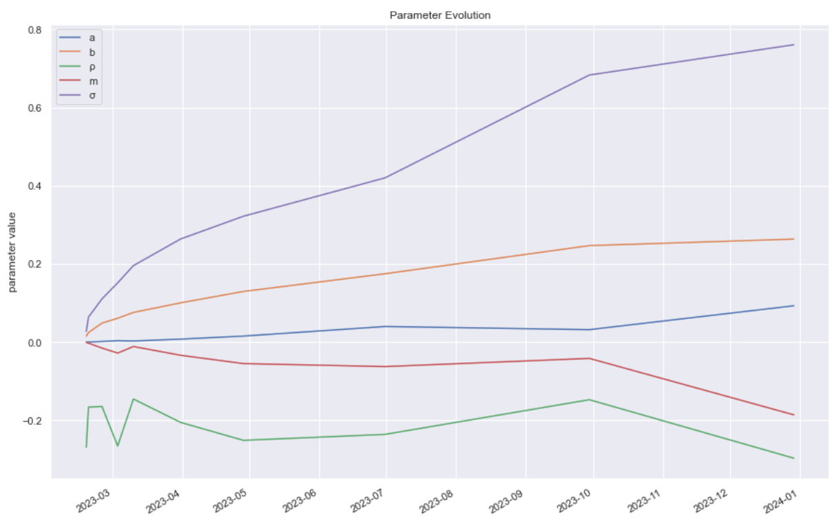
And that pretty much wraps it up. As a parting thought, it is interesting to consider whether the SVI surface calibration can be simplified: in particular, can we fit the entire surface in one go, e.g. by postulating explicit \(\tau\)-dependent expressions for the SVI parameters? The advantage of doing so would go beyond pure parsimony: in particular, it would also do away with the non-trivial issue of how one should interpolate between tenors. I’m not the first person to ponder this problem: Gurrieri, for example, takes a decent shot at postulating such expressions. As always, the devil is in the no-arbitrage detail: Gurrieri’s model is arb free, but only under certain tedious constraints. Whether this ultimately is a successful approach remains to be seen.
Below I have plotted the calibrated parameters for various times to maturity. On a first inspection some of them seem more prone towards simple parametric fits than others. Are there universal laws for how these parameters should behave? How stable is the SVI fit to perturbations in the parameters? Well, these are open questions. You tell me.