An Economist's Guide to the Term Structure of Volatility
Interpreting the vol surface
For anyone who dabbles in options, it is well-known that implied volatility manifestly is not flat, but rather a function of both the strike and the time to maturity: \(\sigma(K,T): \mathbb{R}^+ \times \mathbb{R}^+ \mapsto \mathbb{R}^+\). A priori, the existence of this surface might seem puzzling, but it is not in itself an inconsistency as long as certain no-arbitrage bounds are observed. Still, no-free-lunch arguments do little to explain why the surface is the way that it is. And I bet you won’t be blown away by hand-wavy arguments of supply meeting demand either.
At this point we might interject that the surface is characterised by a number of stylized facts:
- For fixed maturities the surface tends to smile or smirk across the strike domain: i.e. out-of-the-money puts and calls tend to command a vol premium vis-à-vis their at-the-money counterpart. The intuition here is that the hedging demand for tail events in the underlying security drives up option prices in the wings. Viewed from a different angle, recall the Breeden-Litzenberger formula for the risk-neutral transition density: \(f^{\mathbb{Q}}(S_T=K | S_0)=\partial_{KK}^2 C(K,T)\). The volatility smile is effectively the market pricing in the probability of fat-tailed returns (famously, equity options had no smile prior to Black Monday in ‘87).
- For fixed strikes the volatility surface tends to increase with maturity, i.e. the volatility term structure favours contango over backwardation (e.g. futures on the VIX Index exist in a state of contango 70% of the time). The reason for the back-end of the curve being bid up, can again be explained in hedging terms: over longer horizons the market perceives an increased risk of unforeseeable asset price shocks, and long derivative positions are entered accordingly. Note that the slope of the curve simultaneously incentivises investors to enter short vol carry strategies at the front end - a strategy sometimes referred to as “picking up pennies in front of a steam roller”.
Term-time
In this piece I wish to dig a little deeper into the term structure: while I believe the above argument essentially is correct, it misses one key ingredient, viz. the effect of market moving events (be they recurrent (CPI, NFP, ISM,…) or one-off (Brexit, Trump(?), The ETH Merge,…)). To see how this is incorporated it will be helpful to view volatility not as an entity in its own right, but rather as a sum of daily forward volatility components:
\[\sigma_{T} \equiv \sqrt{\frac{1}{T} \sum_{i=1}^T \mathbb{E}_0 [\sigma_{i-1,i}^2]}.\]Intuitively this is appealing because it allows us to think about how much volatility the market expect to materialise on any given day. For example, in the absence of events, imagine that the market prices in a simple mean-reverting (“GARCH(1,1)”) process:
\begin{equation}\label{vmdl} \sigma_{i,i+1}^2 = \theta^2 + \beta(\sigma_{i-1,i}^2 - \theta^2) + \eta_i, \end{equation}
where \(\theta\) is the long-run volatility, \(\beta \in (0,1)\) codifies the speed of mean-reversion, and \(\eta\) is a mean-zero innovation term. Through repeated substitution we find that
\[\begin{aligned} \mathbb{E}_0 [\sigma_{i-1,i}^2] &= \mathbb{E}_0 [\theta^2 + \beta(\sigma_{i-2,i-1}^2 - \theta^2) + \eta_{i-1}] \\ &= \theta^2 + \beta( \mathbb{E}_0[\sigma_{i-2,i-1}^2] - \theta^2) \\ &= \theta^2 + \beta( \mathbb{E}_0[\theta + \beta(\sigma_{i-3,i-2}^2 - \theta^2) + \eta_{i-2}] - \theta^2) \\ &=\theta^2 + \beta^2(\mathbb{E}_0[\sigma_{i-3,i-2}^2] - \theta^2) \\ &= \hspace{3mm}... \\ &= \theta^2 + \beta^{i-1}(\sigma_{0,1}^2 - \theta^2). \\ \end{aligned}\]Remarkably, this rather primitive model of the forward term structure is often sufficient for observable reality, bar a number of spikes associated with event risks. To accommodate these in our model, we write
\[\mathbb{E}_0 [\sigma_{i-1,i}^2] = \theta^2 + \beta^{i-1}(\sigma_{0,1}^2 - \theta^2) + \delta_{i-1,i},\]where \(\delta_{i-1,i} \geq 0\) is an idiosyncratic adjustment for the day. In other words, \(\delta\) captures the excess volatility we expect to induce through the introduction of the event vs. an otherwise “normal” day.
Finally, substituting into for our expression for \(\sigma_T\) we find that the volatility term structure is
\[\sigma_{T} = \sqrt{ \theta^2 + \frac{1-\beta^T}{1-\beta} \cdot \frac{\sigma_{0,1}^2-\theta^2}{T} + \bar{\Delta}_T},\]where \(\bar{\Delta}_T = T^{-1} \sum_{i=1}^T \delta_{i-1,i}\).
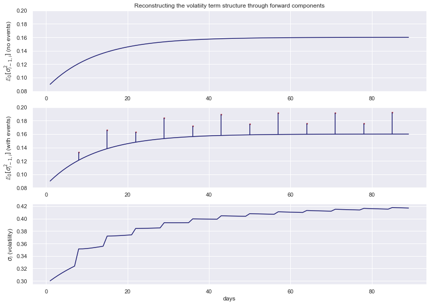
In the example below we consider: (I) a baseline forward volatility term structure with \(\sigma_{0,1}=0.3\), \(\theta=0.4\), and \(\beta=0.92\). (II) The inclusion of two bimonthly events, with respective multiplier effects of 1.1 and 1.2 measured from the baseline. (III) The final volatility term structure, averaging over the forward volatility components.
Extensions
Sometimes a simple monotonic model for the baseline forward term structure is not expressively adequate. E.g. if the forward term structure is spoon shaped, we may take this as an indicator that market prices in reversion to one mean in the short run, and another mean in the long run. Fortunately, this effect is easy to incorporate. In Christoffersen et al. (2008) the following extension to \eqref{vmdl} is proposed:
\begin{equation}\label{vmdl2} \sigma_{i,i+1}^2 = \theta_{i,i+1}^2 + \beta(\sigma_{i-1,i}^2 - \theta_{i-1,i}^2) + \eta_i^{(1)}, \hspace{5mm}
\theta_{i,i+1}^2 = \omega^2 + \rho \theta_{i-1,i}^2 + \eta_i^{(2)}, \end{equation}
in which \(\theta\) in itself has been elevated to a stochastic, mean-reverting process (assume \(\omega>0\) and \(\rho \in (0,1)\)). Through repeated substitution we readily infer that
\[\mathbb{E}_0 [\sigma_{i-1,i}^2] = \omega^2 + \rho^{i-1}(\theta_{0,1}^2 - \omega^2) + \beta^{i-1}(\sigma_{0,1}^2 - \theta_{0,1}^2),\]which we complete by appending a \(\delta\) correction term like before. The volatility term structure can therefore be expressed as
\[\sigma_{T} = \sqrt{ \omega^2 + \frac{1-\rho^T}{1-\rho} \cdot \frac{\theta_{0,1}^2-\omega^2}{T} + \frac{1-\beta^T}{1-\beta} \cdot \frac{\sigma_{0,1}^2-\theta_{0,1}^2}{T} + \bar{\Delta}_T}.\]What I find particularly neat about this model, is its close kinship with the yield curve formula proposed by Nelson and Siegel (1987). To see this, note that in continuous time \eqref{vmdl2} emounts to something like
\[d\sigma_t^2 = d\theta_t^2 + \beta(\theta_t^2 - \sigma_t^2)dt + \eta^{(1)} dW_t^{(1)}, \hspace{5mm} d\theta_t^2 = \rho(\omega^2 - \theta_t^2) dt + \eta^{(2)} dW_t^{(2)},\](yes, this is abuse of notation: the constants you see have been re-defined to keep things simple). Solving for the expected future variance we find
\[\mathbb{E}_0[\sigma_T^2] = \omega^2 + e^{-\rho T}(\theta_0^2 - \omega^2) + e^{-\beta T}(\sigma_0^2 - \theta_0^2)\]or in simple terms:
\[\mathbb{E}_0[\sigma_T^2] = c_1 + c_2 e^{-\rho T} + c_3 e^{-\beta T},\]where the \(c_i\)s are constants. Rewriting \(e^{-\beta T}\) as \(e^{-\rho T}e^{(\rho-\beta) T} \approx e^{-\rho T} (1+(\rho-\beta) T)\) we have to a first order of approximation
\[\mathbb{E}_0[\sigma_T^2] = c_1 + c_2' e^{-\rho T} + c_3' \rho T e^{-\rho T},\]which I submit is equivalent to the Nelson-Siegel definition of the instantaneous forward rate. In particular, solving for \(T^{-1} \int_0^T \mathbb{E}_0[\sigma_t^2] dt\) we obtain an expression for the implied variance at time \(T\):
\[\sigma_{\text{impl},T}^2 = c_1 + c_2' \left( \frac{1-e^{-\rho T}}{\rho T} \right) + c_3' \left( \frac{1-e^{-\rho T}}{\rho T} - e^{-\rho T} \right).\]Conclusion
Viewing the volatility term structure through the lens of forward volatility components with event corrections offers a considerably more economically intuitive approach to volatility. Understanding how these event corrections are determined is an interesting research question, which I will pass over in silence.