A PINN for your Price

Deep Learning with Physics
An oft-repeated exercise is to fit an artificial neural network (ANN) to an array of ex ante given option prices, thereby establishing that multi-parameter non-linear functions can learn the Black-Scholes formula. While numerically pleasing, this fact follows trivially from the Universal Approximation Theorem. Furthermore, it is putting the cart before the horse as it were: ideally we would want our network to price options without giving it access to the very price data we are after. Can it be done?
Thanks to Physics Inspired Neural Networks by Raissi, Perdikaris, and Karniadakis the answer appears to be in the affirmative. Their general idea is as follows: doing theoretical physics effectively boils down to (i) postulating some model, and (ii) solving the governing laws of motion thereof, expressed as partial differential equations with given boundary conditions. Something along the lines of:
\begin{equation}\label{pde} \frac{\partial u(t, \boldsymbol{x})}{\partial t} + \mathcal{D}[u(t, \boldsymbol{x});\boldsymbol{\lambda}] = 0, \end{equation}
where \(u: [0,T] \times \Omega \mapsto \mathbb{R}^d\) is the latent (hidden) solution, and \(\mathcal{D}[u(t, \boldsymbol {x});\boldsymbol{\lambda}]\) is a (possibly non-linear) differential operator parameterised by \(\boldsymbol{\lambda}\), with \(u\) being subject to boundary conditions à la \(u(0,\boldsymbol{x}) = g(\boldsymbol{x})\) et cetera.
Suppose we desire an ANN approximation \(\mathfrak{u}(t, \boldsymbol{x})\) of \(u(t, \boldsymbol{x})\). Traditionally that would entail solving \eqref {pde} first and then feeding the resulting data to the network during its training process. However, as observed by Raissi et al., it may suffice to expose the network to the PDE directly. Specifically, part of the learning objective could be to minimise the mean squared error of \(\mathfrak{f} \equiv \partial_t \mathfrak{u} + \mathcal{D}[\mathfrak{u}; \boldsymbol {\lambda}]\) where the partial derivatives are evaluated using automatic differentiation, for some set of randomly generated coordinates \(\mathbb{F} \equiv \{ (t_i^f, \boldsymbol{x}_i^f) \} \vert_{i=1}^{N_f}\) \(\subset [0,T] \times \Omega\). Meanwhile, we obviously want to respect the boundary conditions: to this end we generate a second set of coordinates \(\mathbb{U} \equiv \{ (t_i^u, \boldsymbol{x}_i^u, u_i^u) \} \vert_{i=1}^{N_u}\) on the boundary, adding to the cost function the mean squared error of the \(\mathfrak{u}\)s (recall, the boundary \(u\)s are known a priori). Altogether, our learning objective is therefore to find the set of neural network parameters \(\{ (\boldsymbol{W}^{[l]}, \boldsymbol{\beta}^{[l]}) \}_{l=0}^K\) which minimises
\[\text{cost} \equiv \frac{1}{N_u} \sum_{i=1}^{N_u} (\mathfrak{u}(t_i^u, \boldsymbol{x}_i^u) - u_i^u)^2 + \frac{1}{N_f} \sum_{i=1}^{N_f} (\mathfrak{f}(t_i^u, \boldsymbol{x}_i^u))^2.\]Raissi et al. go on to demonstrate that they obtain very decent performance for problems pertaining to Burgers’ equation and the Schrödinger equation.
Quants, the most physics envious of all, will surely take heed of this result. In the section below I consider the pricing of European call options using PINNs, and reflect upon the broader viability of the methodology.
Options Pricing with PINNs
Recall that in a Black-Scholes world where the underlying security follows geometric Brownian motion the no-arbitrage price \(u(t,S_t)\) of a European option obeys the PDE
\[\frac{\partial u(t,S)}{\partial t} + r S \frac{\partial u(t,S)}{\partial S} + \tfrac{1}{2} \sigma^2 S^2 \frac{\partial^2 u(t,S)}{\partial S^2} - ru(t,S) = 0,\]where \(r\) is the risk-free rate, and \(\sigma\) is the volatility. For a plain vanilla call option with maturity \(T\) and strike \(K\), the appropriate boundary conditions are \(u(T,S_T) = \max \{S_T - K, 0 \}\), \(u(t,0) = 0\), and \(\lim_{S \rightarrow \infty} u(t,S_t) = S_t - e^{-r(T-t)}K\).
To model this I consider a neural network with ReLU activation functions and three hidden layers, each of size 100 (amounting to 20,601 trainable parameters). The network is implemented in PyTorch with its convenient autograd functionality, and the cost function is optimised using L-BFGS; a quasi-Newton fullbatch gradient-based optimization algorithm. Other parameters are specified below:
config = {
    'params': {'r': 0.04, 'σ': 0.3, 'τ': 1, 'K': 1},
    'layers': [2, 100, 100, 100 , 1] #
}

tsteps = 100 # Number of steps in the time direction
xsteps = 256 # Number of steps in the space direction
N_u = 200 # Number of observable (boundary) points for training. I.e. complete (t,S,C) tuples
N_f = 20000 # Number of randomly generated points
S_min = 1e-20 # min and max space direction
S_max = K * np.exp(-0.5 * σ**2 * τ + σ * np.sqrt(τ) * 3)
τ_min = 0 # min time
Upon training the network for some minutes on my humble laptop, the calibration starts to converge:

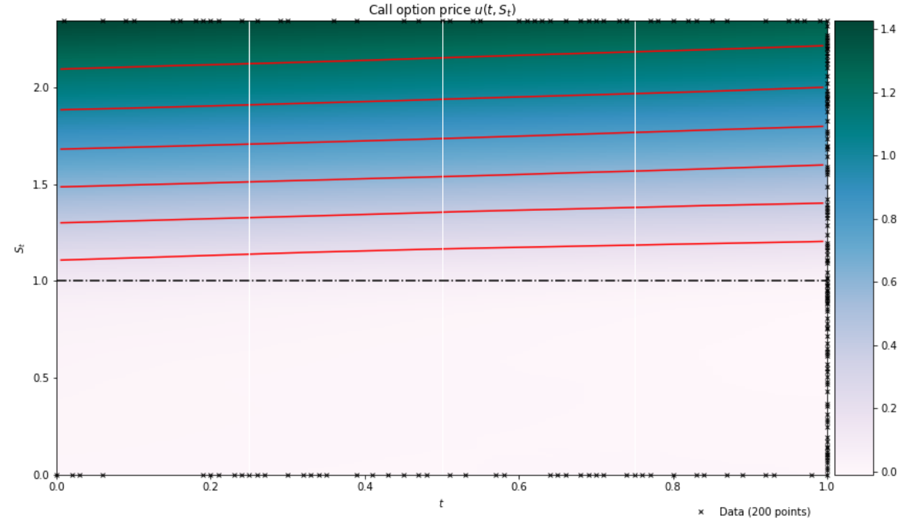
The network understands that deep out-of-the-money options are effectively worthless, while deep-in-the-money options scale as \(\sim S-K\). There is also an appreciation that price levels increase with the time to maturity as shown in the \((t,S_t)\) heatmap below (the red lines are contours; the black line the strike price):
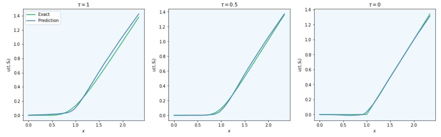
However, that does not mean that the calibration is flawless. For some of the temporal snapshots below, there’s a distinct lack of convexity in the predicted price function.
In fact, there are quite a number of issues with this type of pricing process, including, but not limited to
- The comparative slowness of the procedure vis-à-vis more established numerical methods (Monte Carlo, finite differences).
- The difficulty associated with precluding arbitrage opportunities.
- The sensitivity of the output with respect to neural network architecture, including the choice of activation function.
- Getting stuck in local minima of the cost function.
Nonetheless, I am reasonably excited about the possibilities PINNs bring to quantitative finance: especially in the context of solving non-linear PDEs pertaining to pricing or optimal control (e.g. optimal portfolio problems).
Code Reference
The calibration was done using the code snippets below. The code is a modified version based on work by Raissi et al.. If you find yourself playing around with this stuff and manage to do something interesting/get better fits, I’d like to hear about it!
class DNN(torch.nn.Module):
    """
    A simple class for setting up and stepping through a neural network
    """

    def __init__(self, layers: list):

        super(DNN, self).__init__()

        # parameters
        self.depth = len(layers) - 1

        # set up layer order dict
        self.activation = torch.nn.ReLU

        layer_list = list()
        for i in range(self.depth - 1):
            layer_list.append(
                ('layer_%d' % i, torch.nn.Linear(layers[i], layers[i+1]))
            )
            layer_list.append(('activation_%d' % i, self.activation()))

        layer_list.append(
            ('layer_%d' % (self.depth - 1), torch.nn.Linear(layers[-2], layers[-1]))
        )

        layerDict = OrderedDict(layer_list)

        # deploy layers
        self.layers = torch.nn.Sequential(layerDict)

    def forward(self, x: torch.Tensor) -> torch.Tensor:

        out = self.layers(x)
        return out
class PhysicsInformedNN():
    """
    Physics inspired neural network for Black Scholes
    For other PDEs adjust self.net_f and input values
    """

    def __init__(self, X_u: np.ndarray,
                         u: np.ndarray,
                         X_f: np.ndarray,
                         config: dict,
                         lb: np.ndarray,
                         ub: np.ndarray):

        # boundaries
        self.lb = torch.tensor(lb).float().to(device)
        self.ub = torch.tensor(ub).float().to(device)

        # data
        self.x_u = torch.tensor(X_u[:, 0:1], requires_grad=True).float().to(device)
        self.t_u = torch.tensor(X_u[:, 1:2], requires_grad=True).float().to(device)
        self.x_f = torch.tensor(X_f[:, 0:1], requires_grad=True).float().to(device)
        self.t_f = torch.tensor(X_f[:, 1:2], requires_grad=True).float().to(device)
        self.u = torch.tensor(u).float().to(device)

        # network configurations
        self.layers = config['layers']
        self.params = config['params']

        # deep neural networks
        self.dnn = DNN(self.layers).to(device)

        # optimizers: using the same settings
        self.optimizer = torch.optim.LBFGS(
            self.dnn.parameters(),
            lr= 0.1, #1.0,
            max_iter=50000,
            max_eval=50000,
            history_size=50,
            tolerance_grad=1e-5,
            tolerance_change=1.0 * np.finfo(float).eps,
            line_search_fn="strong_wolfe"       # can be "strong_wolfe"
        ) # https://en.wikipedia.org/wiki/Limited-memory_BFGS

        #
        self.iter = 0
        self.ierr = {}

    def _net_u(self, x, t):
        """ boudary: nn value """
        return self.dnn(torch.cat([x, t], dim=1))

    def _net_f(self, x, t):
        """ interior: nn PDE """

        u = self._net_u(x, t)
        u_t = torch.autograd.grad(
            u, t,
            grad_outputs=torch.ones_like(u),
            retain_graph=True,
            create_graph=True
        )[0]
        u_x = torch.autograd.grad(
            u, x,
            grad_outputs=torch.ones_like(u),
            retain_graph=True,
            create_graph=True
        )[0]
        u_xx = torch.autograd.grad(
            u_x, x,
            grad_outputs=torch.ones_like(u_x),
            retain_graph=True,
            create_graph=True
        )[0]

        return u_t + self.params['r']*x*u_x + 0.5*pow(self.params['σ'],2)*x*x**u_xx - self.params['r']*u

    def _loss_func(self):

        self.optimizer.zero_grad()

        u_pred = self._net_u(self.x_u, self.t_u)
        f_pred = self._net_f(self.x_f, self.t_f)
        loss_u = torch.mean((self.u - u_pred) ** 2)
        loss_f = torch.mean(f_pred ** 2)

        loss = loss_u + loss_f

        loss.backward()
        self.iter += 1

        if self.iter % 10 == 0:
            print(
                'Iter %d, Loss: %.5e, Loss_u: %.5e, Loss_f: %.5e' % (self.iter, loss.item(), loss_u.item(), loss_f.item())
            )

        self.ierr[self.iter] = {'loss': loss.item(), 'loss_u': loss_u.item(), 'loss_f': loss_f.item()}

        return loss

    def train(self):

        self.dnn.train()
        self.optimizer.step(self._loss_func)

    def predict(self, X: np.ndarray) -> tuple:
        x = torch.tensor(X[:, 0:1], requires_grad=True).float().to(device)
        t = torch.tensor(X[:, 1:2], requires_grad=True).float().to(device)

        self.dnn.eval()
        u = self._net_u(x, t)
        f = self._net_f(x, t)
        u = u.detach().cpu().numpy()
        f = f.detach().cpu().numpy()
        return u, f